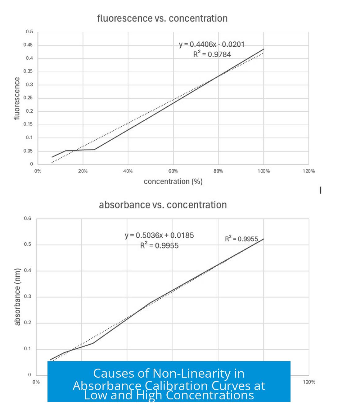
Why Do Calibration Curves of Absorbance Versus Concentration Deviate from a Straight Line When a < 0.1 and When a > 1?
Calibration curves deviate from linearity at very low absorbance (a < 0.1) due to instrumental noise and baseline errors, and at high absorbance (a > 1) primarily because of stray light interference and chemical effects that alter absorptivity.
Understanding Calibration Curves in Absorbance Spectroscopy
Calibration curves plot absorbance against analyte concentration, ideally forming a straight line described by Beer-Lambert Law. This law predicts proportionality between absorbance and concentration within certain bounds.
Deviations arise outside this optimal absorbance range. Instruments and chemical phenomena impose practical limitations affecting accuracy.
Deviations at Low Absorbance (a < 0.1)
Instrumental Limitations and Baseline Noise
At absorbance values below 0.1, measurements suffer increased error. Small fluctuations in baseline signals impact results proportionally more. For example, differences in light path length in dual beam spectrophotometers cause variability.
- Baseline drift represents a larger fraction of signal.
- Electronic noise becomes significant compared to the weak absorbance signal.
- Such noise impacts both accuracy and precision of absorbance readings.
Signal-to-Noise Ratio Issues
When concentration is very low, the absorbance approaches the detection limit of the spectrophotometer. The signal from the analyte is close in magnitude to noise and solvent background.
This leads to uncertain measurement of absorbance difference, causing the calibration curve to flatten or scatter at the lower end.
Sensitivity Limit of Instruments
While most spectrophotometers measure absorbance down to approximately 0.005, practical difficulties arise near this threshold. Below 0.1 absorbance, the instrument may not reliably distinguish the weak signal from background noise.
Such limitations make the calibration curve deviate from linearity at low concentrations.
Conceptual Analogy: Underestimation at Low Concentrations
Imagine trying to estimate a sparse crowd by the chance of observing others. Low analyte concentration means fewer photon absorptions. This sparsity leads to underestimation, analogous to “not seeing enough people,” which forms a nonlinear curve.
Deviations at High Absorbance (a > 1)
Effect of Stray Light
At high absorbance, only a small fraction of light passes through the sample. The light reaching the detector is near the instrument’s detection threshold.
Stray light—unwanted light entering the detector from reflections or scattering inside the instrument—comprises a significant portion of detected light. This causes measured absorbance to saturate and flatten, as the instrument registers this stray light as transmitted light.
Reducing path length lowers absorbance, extending linear response, but stray light remains a limiting factor.
Chemical and Physical Causes of Nonlinearity
High analyte concentration can alter the optical properties of the solution:
- Molecular interactions modify absorptivity.
- Changes in solvent polarity or pH affect absorption spectra.
- Aggregation or scattering alters effective absorbance.
These factors break the linear relationship expected from diluted solutions.
Optical Density and Saturation Effects
When absorbance approaches or exceeds 1, the solution appears very dark. Most light is absorbed or scattered, limiting further changes measured by the detector.
This saturation effect causes the calibration curve to “shallow out” at high concentration.
Conceptual Analogy: Overestimation at High Concentration
Consider a dense crowd blocking your view; you cannot accurately count people and may overestimate. Similarly, at high analyte concentration, absorbance readings saturate and sometimes overstate absorption due to scattered light appearing as transmitted light.
Role of Path Length
Shortening the path length reduces the effective absorbance, pushing high-concentration values into the linear range of the instrument.
For example, microvolume spectrophotometers with 1 mm path length multiply readings to report standard 10 mm path length absorbance. This can improve measurement within 1–10 AU but does not prevent chemical deviations from Beer-Lambert Law.
General Considerations
Instrument and Sample Dependency
The absorbance limits for linearity depend on many factors:
- Instrument sensitivity and optical design.
- Light source stability and detector response.
- Sample properties including solvent, matrix, and analyte behavior.
- Path length of the cuvette or cell.
Hence, commonly accepted thresholds of 0.1 and 1 absorbance units are approximate. Users should determine the limits of detection (LOD), limits of quantitation (LOQ), and limits of linearity (LOL) for each system.
Mathematical Background of Absorbance
Absorbance (A) relates to transmittance (T) by A = -log(T). Low absorbance corresponds to high transmittance. For example:
- A = 0.1 → T ≈ 0.79 (79% light passes)
- A = 1.0 → T = 0.1 (10% light passes)
- A = 2.0 → T = 0.01 (1% light passes)
At very high absorbance, almost no light reaches the detector. Stray light and noise dominate the signal, causing curve flattening.
Summary of Causes of Non-Linearity in Calibration Curves
| Absorbance Range | Causes of Deviation | Key Effects |
|---|---|---|
| < 0.1 |
|
|
| > 1 |
|
|
Takeaways
- Calibration curves deviate at low absorbance (<0.1) due to signal noise and baseline errors.
- At high absorbance (>1), stray light and chemical interactions cause nonlinear responses.
- Instrument sensitivity, sample properties, and path length affect these limits.
- Users should validate the linear range and report detection and linearity limits.
- Appropriate sample dilution or path length adjustment extends the linear range.


Leave a Comment