Interpreting Protein Assay Standard Curves: A Comprehensive Guide to Success in Your Lab

Interpreting Protein Assay Standard Curves

Protein assay standard curves serve as essential tools to quantify protein concentration from absorbance data. These curves plot known protein concentrations against corresponding absorbance values, establishing a reference for measuring unknown samples.

Creating and Using the Standard Curve

Plotting the Standard Curve

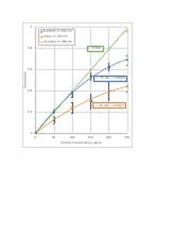
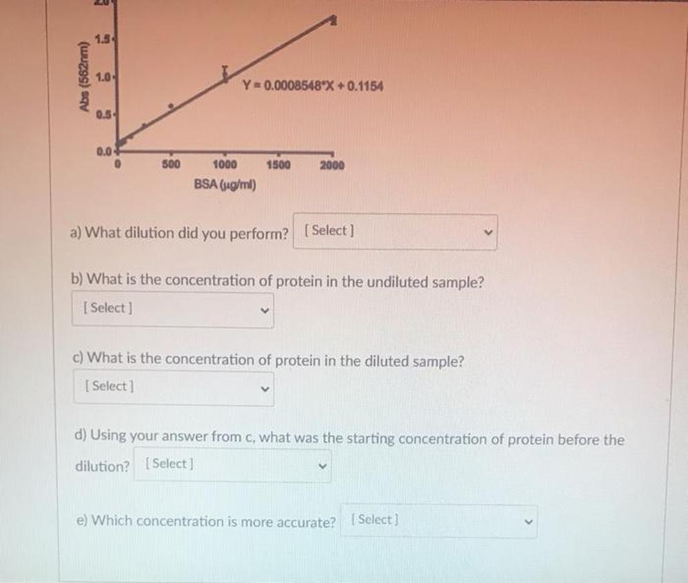
Start by measuring absorbance for a series of known protein concentrations (standards). Plot concentration on the x-axis and absorbance on the y-axis. The resulting graph should be linear within a specific range. Apply a linear regression to obtain the trend line equation, which relates concentration (conc) and absorbance (abs).

Rearranging the Trend Line Equation

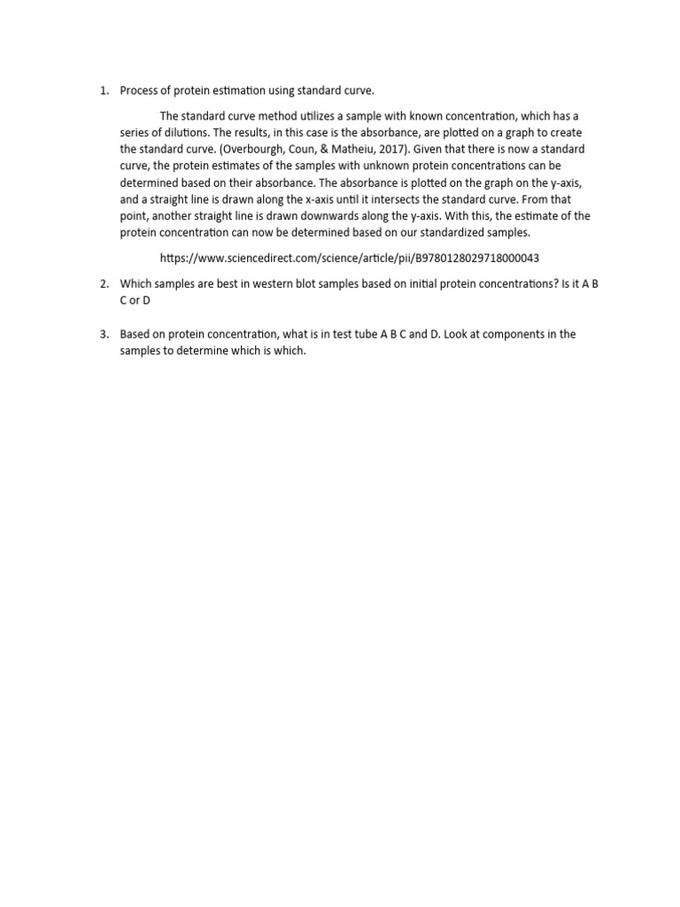
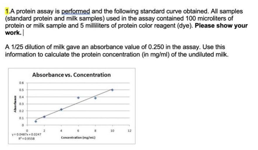
Typically, the trend line equation has concentration as the independent variable and absorbance as the dependent variable (e.g., abs = m × conc + b). For practical use, rearrange this equation to express concentration as a function of absorbance: conc = (abs – b) / m. This allows direct calculation of protein concentration from measured absorbance values.

Calculating Protein Concentration from Sample Absorbance

Measure the absorbance of your unknown protein sample. Insert this absorbance into the rearranged equation to determine the protein concentration. Accuracy depends on ensuring the sample’s absorbance falls within the established linear range of the standard curve.

Characteristics and Considerations of the Standard Curve

Linearity Range

The standard curve maintains linearity only within a certain protein concentration range. Beyond this, dye saturation occurs, causing the absorbance signal to plateau. Exceeding this range can lead to inaccurate concentration estimates.

Absorbance Dependence on Protein Concentration

Absorbance directly depends on protein concentration due to the binding of dye molecules to proteins. This relationship underlies the assay’s quantitative capability and justifies the linear model within the valid range.

Determining Unknown Sample Concentration

To find an unknown concentration, identify the sample’s absorbance on the y-axis of the standard curve. Then locate the corresponding concentration on the x-axis. Use the trend line equation to ensure precision, especially if the value lies between plotted standards.

Recommended Formula for the Assay

While a linear equation suffices in many cases, assay providers may recommend a three-parameter formula to better fit the data, especially when nonlinear regions are present. This approach improves accuracy over a broader range.

Key Takeaways

• Plot a standard curve with known protein concentrations against absorbance.
• Obtain and rearrange the trend line equation to calculate concentration from absorbance.
• Ensure sample absorbance values fall within the curve’s linear range.
• Recognize absorbance depends on protein concentration and dye binding.
• Consider a three-parameter formula for more precise curve fitting if necessary.

Mastering the Art of Interpreting Protein Assay Standard Curves

Interpreting protein assay standard curves means turning your experimental data into a reliable measure of protein concentration. Sounds straightforward, right? Well, it can be—if you know the tricks and pitfalls. Let’s dive into the nuts and bolts of this essential lab skill.

Imagine you’ve run a protein assay, and now your spectrophotometer spits out some absorbance (abs) numbers for your sample. What’s next? Do you guess the protein content? No! You grab your trusty standard curve and let it do the heavy lifting.

Creating the Standard Curve: Your Protein Detective’s Map

The first step is plotting your standard protein concentrations against their absorbance values. On your graph, the x-axis is the known concentration of the protein standards, while the y-axis shows the measured absorbance. This plot should ideally give you a straight line—our best friend in quantification.

Why a straight line? Because within certain limits, absorbance is directly proportional to protein concentration. Your trend line, generated from this plot, represents this relationship mathematically. Typically, a linear regression gives an equation in the form:

y = mx + b

Here, y is absorbance, x is concentration, m is the slope, and b is the y-intercept.

Rearranging the Equation to Solve Protein Mystery

Okay, you have the equation, but there’s a catch. To find protein concentration from an unknown sample’s absorbance, you need the equation flipped. Instead of absorbance as output, concentration becomes the output. So, rearrange the equation to:

x = (y – b) / m

Here, x (concentration) depends on your measured absorbance y. This step is crucial to translate the reading into something meaningful. It’s like converting a foreign language to your native tongue.

Plugging in Sample Absorbance: The Moment of Truth

With the rearranged formula, you now input your sample’s absorbance reading. The equation spits out the protein concentration. This simple substitution turns raw spectrometer outputs into figures you can trust—and data your research depends on.

The Linearity Range: Sweet Spot or Danger Zone?

A quick word of caution: your standard curve is linear only within a certain protein concentration range. Push beyond this, and the dye used in the assay saturates. Saturation means the absorbance won’t increase with protein concentration anymore—which can give you misleading results.

So, when you prepare your standards, pick a concentration range that matches your expected sample levels. If your sample absorbs light beyond the curve’s linear region, dilute it, then measure again.

Absorbance Depends on Protein Concentration—But What About Other Variables?

It’s tempting to think that absorbance always reflects protein concentration perfectly. In reality, absorbance can be influenced by other factors like the type of protein, assay conditions, and the presence of interfering substances. So always keep your assay conditions consistent and include proper controls.

Mapping Unknowns Back to the Standard Curve

So, you have an unknown absorbance. What do you do with it? Locate its position on the y-axis (absorbance) of your standard curve graph. Trace horizontally across to the curve, then drop down vertically to the x-axis to find the corresponding protein concentration. This graphical method complements your formula-based calculation and is a good visual check.

The Recommended 3-Parameter Formula: When Simple Isn’t Enough

Basic linear equations work for many protein assays, but sometimes the standard curve isn’t perfectly linear. Here, a 3-parameter formula comes to the rescue. This method accounts for the curve’s shape more accurately, especially near saturation zones.

The 3 parameters typically involve:

• Min absorbance baseline (background)
• Max absorbance plateau (dye saturation)
• Curve steepness (sensitivity to concentration changes)

This formula fits your data better, giving more precise concentration values across a broader range. While it’s a bit more complex, software tools usually handle the heavy math.

Why Should You Care? Practical Insights and Takeaways

Interpreting protein assay standard curves accurately impacts your research credibility. Imagine publishing results based on inflated protein concentrations because your sample was saturated. Ouch.

On the flip side, mastering this technique equips you with a powerful tool to quantify proteins efficiently and reproducibly. Whether you’re studying enzymes, antibodies, or general protein content, your data gains scientific rigor.

A Personal Lab Tale

Years ago, I botched a protein quantification: my samples were too concentrated, and the absorbance readings hit the top of the scale. Blindly trusting linear regression, I reported ridiculously high concentrations. A colleague’s advice to check dye saturation saved me embarrassment. We diluted samples, re-measured, and got plausible values. That experience taught me to respect the standard curve’s limits—an invaluable lesson!

Final Recommendations for Protein Assay Success

1. Always prepare a fresh standard curve with each assay batch.
2. Choose standard concentrations wisely, covering expected sample ranges.
3. Check that absorbance readings lie within the linear region.
4. Consider a 3-parameter fit if saturation or non-linearity appears.
5. Replicate measurements for accuracy and consistency.

In summary, interpreting protein assay standard curves means combining careful plotting, smart equation rearranging, and awareness of assay limitations. With these skills, protein quantification becomes less of a guessing game and more of a precise science.

So, next time you face a stack of absorbance numbers, remember: your standard curve is there to guide you—just read it right!